Unit VI Lesson 1

Direction Fields

Construction of direction fields (slope fields) along isoclines of a differential equation.
Example of a direction field, constructed automastically, but description of how to make one manually, and solutions drawn on a slope field.
Another example of a direction field with solutions drawn on the field.

In this section, we look at ways to get the graph of the solution of a differential equation without solving the equation. I think it is best to tell you now at the end of the course that only a small portion of naturally occuring differential equations can be solved through the traditional means that we have seen thus far. Other methods we are about to discuss are frequently used.

Suppose we have a first order differential equation

Then on the curve f(x,y)=c, the slopes of the tangent lines for the solution of the differential equation are the same (in fact the are all c).

Def: isoclines

The curves f(x,y)=c are called isoclines of the DE

They are curves in which the inclination of the tangent lines (-cline) is the same (iso-).

If we would draw small ‘lineal elements’ (line segments) representing the tangent lines at points along an isocline, we would be drawing a direction field (also called slopefield) of

You can think of the direction field as a fingerprint of the function y that is the solution to the DE.

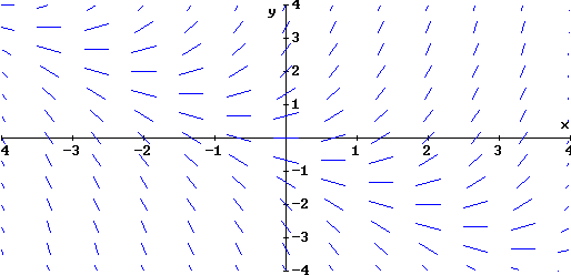
Example

The isoclines are lines with slope=-1 since y=-x+c and different y intercepts, and the y intercepts give the value of the slope. Along x+y=2, for instance, the slope is 2. The direction field is shown here:

Some possible solutions of the differential equation are sketched below. The sketches are reasonable approximations to graphs of solutions, since the lineal elements are snapshots of the tangent lines to the graph of the solution.

Comment: I used the Derive CAS to produce this picture by loading the file Ode_appr.mth to get the direction field and ode1.mth to get the solution of the DE. You need to adjust the range of the graph, and watch out for plot colors as well to get the same effect. These can be done by hand, and that is acceptable, but tedious.

Try one here, then take the link to compare.

Ex1. Draw the direction field, then sketch a few possible solutions for the differential equation:

Take this link after trying it yourself.

****assignment****
Chapter 2 Section 1
Problems 1,3,7,9